Tensile and Compressive Axial Loading

In this text you will learn:
- when we are dealing with tensile loading
- about the convention of positive sign for normal force
- what is and what is the formula for:
a) elongation of a rod
b) deformation of a tensile rod
c) normal stress
- what is Poisson's ratio
- what is the form of stress and strain tensor for a tensile rod
- how to calculate the elastic energy for a tensile rod
- how the stress cube and Mohr's circle look like in the case of axial tension

You will also find calculation examples and video courses at the bottom of the page as well as

When are we dealing with axial tensile loading?

Axial tensile/compressive loading of a rod occurs when all the forces acting on the cross-section from one side add up in such a way that they create a single force perpendicular to the cross-section. This force acts along the axis of the rod and is attached at its center of gravity.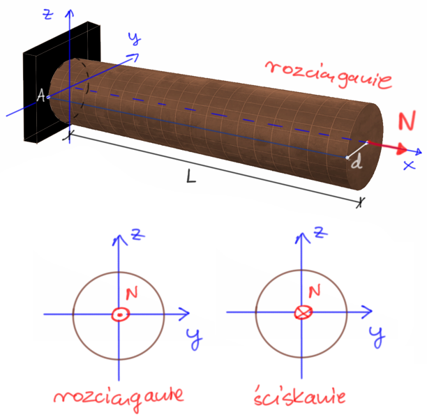

Fig1. Axial tensile loading of a circular rod

Convention of positive sign for normal force

If the direction of this force is the same as the normal (perpendicular) to the outer surface of the rod, we call it tensile force, and we assign it a positive sign for its values.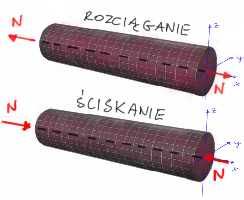

Fig2. Sign convention for normal/axial forces

The elongation of a rod or its part is calculated as follows:

The total change in length of the rod is defined as the integral (with respect to length) of the longitudinal strain function:
\[ \Delta l=\int_0^l \varepsilon_x d x=\int_0^l \frac{N(x)}{E A} d x \] If we are dealing with a homogeneous rod with a specified stiffness for tension (\(EA=\) const \()\) subject to a normal force of constant value \((N=\) const \()\), and not a force function, which may be associated, for example, with the consideration of its own weight, we obtain:
\[ \Delta l=\int_0^l \frac{N}{E A} d x=\frac{N}{E A} \int_0^l d x=\frac{N l}{E A} . \]
where:
N - normal force or N(x) - force function
l - length of the rod or part of the rod
E - Young's modulus (material constant)
A - cross-sectional area

Deformation of a tensile rod

a) Effect of static loading

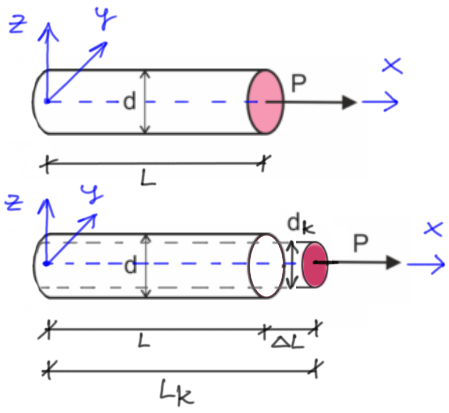
Fig3. Elongation of a rod and change of dimensions

Longitudinal strain \( \varepsilon_x \) and transverse strains \( \varepsilon_y , \varepsilon_z \)
are calculated as follows:
\[ \varepsilon_x=\frac{\Delta L}{L}=\frac{L_f-L}{L} \] \[ \varepsilon_y=\frac{\Delta d}{d}=\frac{d_f-d}{d} \] \[ \varepsilon_z=\frac{\Delta d}{d}=\frac{d_f-d}{d} \]

b) Effect of non-static loading

The length of the rod can also change due to non-static effects, such as uniform heating of the rod compared to its initial temperature (installation temperature). Thermal strains resulting from the evenly heating or cooling of the rod are expressed by the formula: \[ \varepsilon_{x(T)}=\alpha_t \cdot t_0 \] \( \quad \) where:
\( \quad \) - \(t_0\) - difference in temperature of the rod compared to its original temperature expressed in Kelvin \( [K] \) or Celsius degrees \( [^oC] \) (the temperature difference in both scales is always the same)
\( \quad \) - \( \alpha_t \) - coefficient of thermal expansion, defined as the unit change in length caused by a change in temperature of \( 1K / 1^oC \) expressed in \( \frac{1}{K} \) or \( \frac{1}{^oC} \)

The change in length of the rod with length \(l\) under the influence of a uniform temperature is expressed by the formula: \[ \Delta l_T=\varepsilon_{x(T)} \cdot l=\alpha_t \cdot t_0 \cdot l \] So if the rod is subject to static and thermal loads, then we can write: \[ \Delta l=\Delta l_N+\Delta l_T=\int_0^l \frac{N(x)}{E A} d x+ \alpha_t \cdot t_0 \cdot l \]
The relationship between longitudinal and transverse strains is determined by the Poisson's ratio
The change in volume is calculated from the relation: \( \Delta V=(ε_x+ε_y+ε_z)\cdot V \)
V - initial volume of the rod

Poisson's Ratio

Poisson's ratio is a material physical constant that describes the relationship between transverse strain (change in width) and longitudinal strain (change in length) in a material.
Specifically, Poisson's ratio (usually denoted by \( \nu \) ) is the ratio of transverse strain to longitudinal strain in a material.
It is expressed as:
\[ \nu = - \frac{ε_{transverse}}{ε_{longitudinal}} \] where:
\( \quad \nu \) is Poisson's ratio,
\( \quad ε_{transverse} \) is the transverse strain,
\( \quad ε_{longitudinal} \) is the longitudinal strain.

In the above example, we would write:
\[ \nu = - \frac{ε_y}{ε_x} \] \[ \nu = - \frac{ε_z}{ε_x} \] or transforming:
\[ ε_y = -ν \cdot ε_x \] \[ ε_z = -ν \cdot ε_x \] The Poisson's ratio is important in the analysis of material strength because it allows to determine how the material behaves under load, especially in terms of its elasticity and resistance to deformation.
Different materials have different Poisson's ratios, which affect their mechanical properties and behavior under load. For example, for some materials, ν is close to 0, which means that changes in one direction (transverse) are practically imperceptible in case of deformations in another direction (longitudinal).
In other materials, ν can be larger, which means greater variation in those deformations.

Normal stresses

Fig. 4. Distribution of normal stresses

The formula for normal stresses in axial tension/compression at any point of the cross section is as follows: \[ \sigma=\frac{N}{A} \] where:
N - normal (axial) force,
A - cross-sectional area of the rod.

Form of stress and strain tensors for axially tensioned/compressed rod:

\begin{aligned} T_\sigma=\left[\begin{array}{ccc} \sigma_x & 0 & 0 \\ 0 & 0 & 0 \\ 0 & 0 & 0 \end{array}\right] \quad T_{\varepsilon}=\left[\begin{array}{ccc} \varepsilon_x & 0 & 0 \\ 0 & \varepsilon_y & 0 \\ 0 & 0 & \varepsilon_z \end{array}\right] \end{aligned}

Strain energy for axially tensioned/compressed rod

For a rod with a single characteristic interval: \[U=\int_0^L \frac{N^2(x)}{2 E A} d x\] For a rod with multiple intervals (if the cross section or material changes along the length of the rod or if there are axial forces at different locations) then we need to sum up over all characteristic intervals: \[U=\sum_{i=1}^n \int_0^{L_i} \frac{N_i^2(x)}{2 E_i A_i} d x\]

Stress cube for the case of axial tension/compression, principal stresses and directions, Mohr circle

If we are dealing with tension, then the stress \( \sigma_1=\frac{N}{A} \) is the maximum stress, i.e. the principal stress. The minimum stress is \( \sigma_2=0 \).
If we are dealing with compression, then the stress \( \sigma_2=\frac{-N}{A} \) is the minimum stress, i.e. the principal stress. The maximum stress is \( \sigma_1=0 \).
The shear stresses are equal to 0.

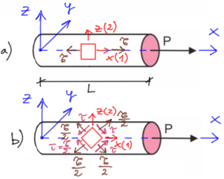
Fig. 5. Stress cubes for tension
a) principal stresses
b) cube rotated by 45 degrees - state with maximum shear stresses

Let's consider the cross section inclined at an angle of \( 45^o \) to the axis of the rod, because in this cross section there are maximum shear stresses in the axially tensioned/compressed rod.
The formula for the maximum and minimum shear stresses in a planar state of stress is as follows: \[ \begin{aligned} & \tau_{\max }=\frac{\sigma_{1}-\sigma_{2}}{2}=\frac{\sigma}{2}, \\ & \tau_{\min }=-\frac{\sigma_{1}-\sigma_{2}}{2}=-\frac{\sigma}{2} \end{aligned} \] How do we know that the maximum shear stress in this case occurs at an angle of \( 45^o \)?
If we know that the value of the maximum shear stress is \( \tau_{max}=\frac{\sigma}{2} \) and that \( \sigma_1=\sigma \) and \( \sigma_2=0 \), where \( \sigma=\frac{N}{A} \), we can use the formula describing the state of stress in a cross section inclined at an angle \( \alpha \) to the direction of the larger principal stress: \[ \tau_\alpha=\frac{\sigma_1-\sigma_2}{2} \cdot \sin (2 \alpha) \] substituting the data: \[ \frac{\sigma}{2}=\frac{\sigma-0}{2} \cdot \sin (2 \alpha) \quad |:\frac{\sigma}{2} \] \[ 1=\sin (2 \alpha) \quad | asin ( ) \] \[ asin (1) = 2 \alpha \] \[ 90^o = 2 \alpha \] \[ \alpha = 45^o \] What are the normal stresses in the cross section rotated by \( 45^o \)? This is determined by the formula: \[ \sigma_\alpha=\sigma_1 \cos ^2 \alpha+\sigma_2 \sin ^2 \alpha=\frac{\sigma_1+\sigma_2}{2}+\frac{\sigma_1-\sigma_2}{2} \cos (2 \alpha) \] substituting the data: \[ \sigma_\alpha=\sigma \cos ^2 (45^o) +0 \cdot \sin ^2 \alpha=\frac{\sigma}{2} \]

Mohr's circle

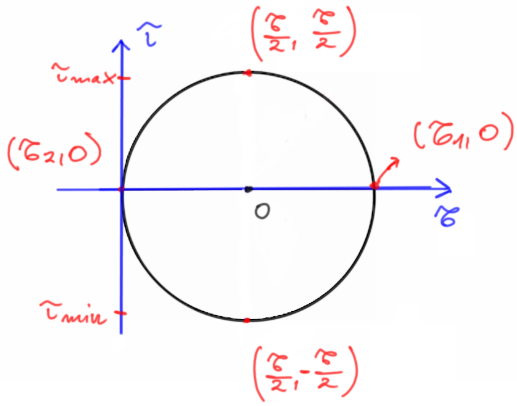
Fig. 6. Mohr's circle - axial tension

Now let's move from theory to practice

We have a lot of free video courses on this topic, which you can find below.
Click on the text below the thumbnail to scroll to the exercise you are interested in.

Single rods - statically determinable systems	Systems of rods - statically determinable	Indeterminable statics exercises
ZADANIE 1	ZADANIE 4	ZADANIE 7
ZADANIE 2	ZADANIE 5	ZADANIE 8
ZADANIE 3	ZADANIE 6	ZADANIE 9